FrediFizzx wrote: ↑Thu Dec 16, 2021 4:32 am
Perhaps for lurkers I should explain the fairly simple Mathematica code for this model. Joy, jump in if I don't get something quite right.
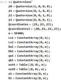
This first section of code is setting up the quaternion package and a method for creating quaternions from scalar values and vector coordinates. Then "m" is just the number of trials or events that will be done in the simulation. The rest are just storage containers for event values of the different parts of the simulation. A note about quaternions here; Mathematica basically treats quaternions as a scalar plus a 3D vector. IOW, the first element in the quaternion is the scalar.
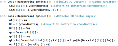
Then we have the Do-loops. The first line makes a unit vector "s" and gives us the x, y and z values of the surface of a unit sphere. It is the same for the vectors "a" and "b". The next two lines makes two quaternions that represent the spins of the two singlet particles. One having opposite spin from the other. Then on the A Do-loop we have the vector "a" being generated and the next line is so that the values of "a" can be taken past the Do-loop. Then Da is the detector quaternion for the A side. It's a quaternion because it can be rotated. Then again we make Da1 so the values can be taken past the Do-loop. The "qa" is another quaternion that is formed by the detector quaternion and the particle quaternion that is being detected. Then "qA" is the result of applying the full polarization to the quaternion "qa". It will have the value +/-1. The limit replacement function is the same function as sign(qa) but has more explanation power as to what is happening in the detection process. Then the values of "a" and "qA" are collected in outA and we see that the Do-loop is iterated "m" times. The B side is the same as the A side only with the B values.
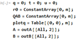
Then we have some more container setup and the A and B output values are extracted from outA and outB. We will take a break here in case we have questions or comments so far before we get into the long section. Which I will do in a while. A note for Lurkers; you can post comments or questions as a guest (you don't have to register).
Now, for the long section.
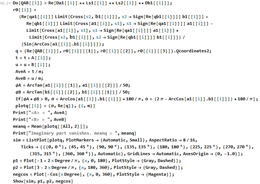
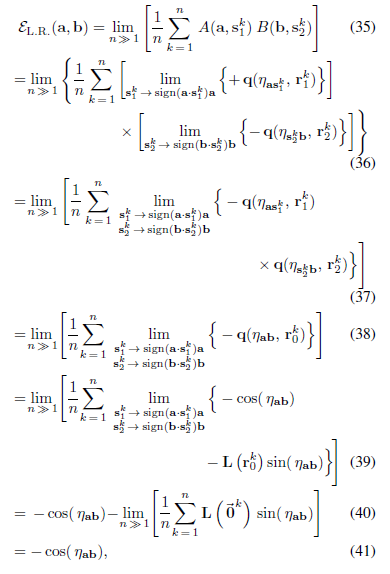
In the first line, QAB is the real part of the product of the A side with the B side. IOW, it is a scalar and is actually equal to the value of
-a.b for the "i"th event. However, that product also leaves us with an imaginary part of the quaternion which we must get rid of like in the following.
In[41]:= Da1[[1]]**Ls1[[1]]**Ls2[[1]]**Db1[[1]]
Out[41]= Quaternion[0.349095, -0.697829, 0.387371, 0.491031]
Then the next line for r0 you will need to look at Joy's analytical formulas. We take the limits of the A and B side quaternions which ends up forming a null vector r0 = {0,0,0} for every event. Then the line with q =, we form a quaternion with QAB and r0. This makes the imaginary "residue" gone so that we only end up with values for
-a.b per event. We didn't need the r_1 and r_2 vectors like in Joy's analytical formulas because they are already contained within the involved quaternions.
The rest is pretty self-explanatory but ask questions if there is something not understood.
.